CS173: Intro to Computer Science - Purple America (100 Points)
Assignment Goals
The goals of this assignment are:- To manipulate String variables in common ways using practical data found on the web for a meaningful purpose.
- To use iteration to facilitate the rendering of many counties in a graphical display
- To use the HashMap data structure for storing associated key-value pairs
- To use the ArrayList data structure as a generic container
- To utilize library functionality from external jar files and build upon existing functionality
The Assignment
If (and only if) you are using GitHub to submit, you can clone this assignment from GitHub Classroom at https://classroom.github.com/a/E9q6QJNl. Otherwise, you may skip this step!In the United States, many elections, including the presidential election, are decided by a “winner-take-all” system via a “first-past-the-post” model. In this model, people in a region cast votes for their candidate of choice among a set of candidates. Whichever candidate receives the plurality of votes cast “wins” the election. In American presidential elections, winning a particular region results in receiving a number of “Electoral College” votes; in many states, all of the electoral college votes are cast for the candidate who won the “first-past-the-post” vote in that state.
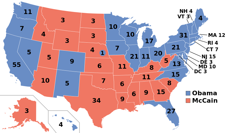
This results in an electoral map like the one below from the 2008 United States presidential election, in which information is lost pertaining to the margin of victory. For example, it is known that President Obama won the Commonwealth of Pennsylvania in 2008 (due to the blue color), receiving its 21 electoral college votes; similarly, it is known that Senator McCain won the state of Texas (due to the red color) and received its 34 electoral college votes. It is not known from this visualization, however, whether these states were won by a single vote or by a landslide. For this reason, it is important to carefully choose visualizations that convey as much information as possible, and to be clear about the limitations of the visualization.
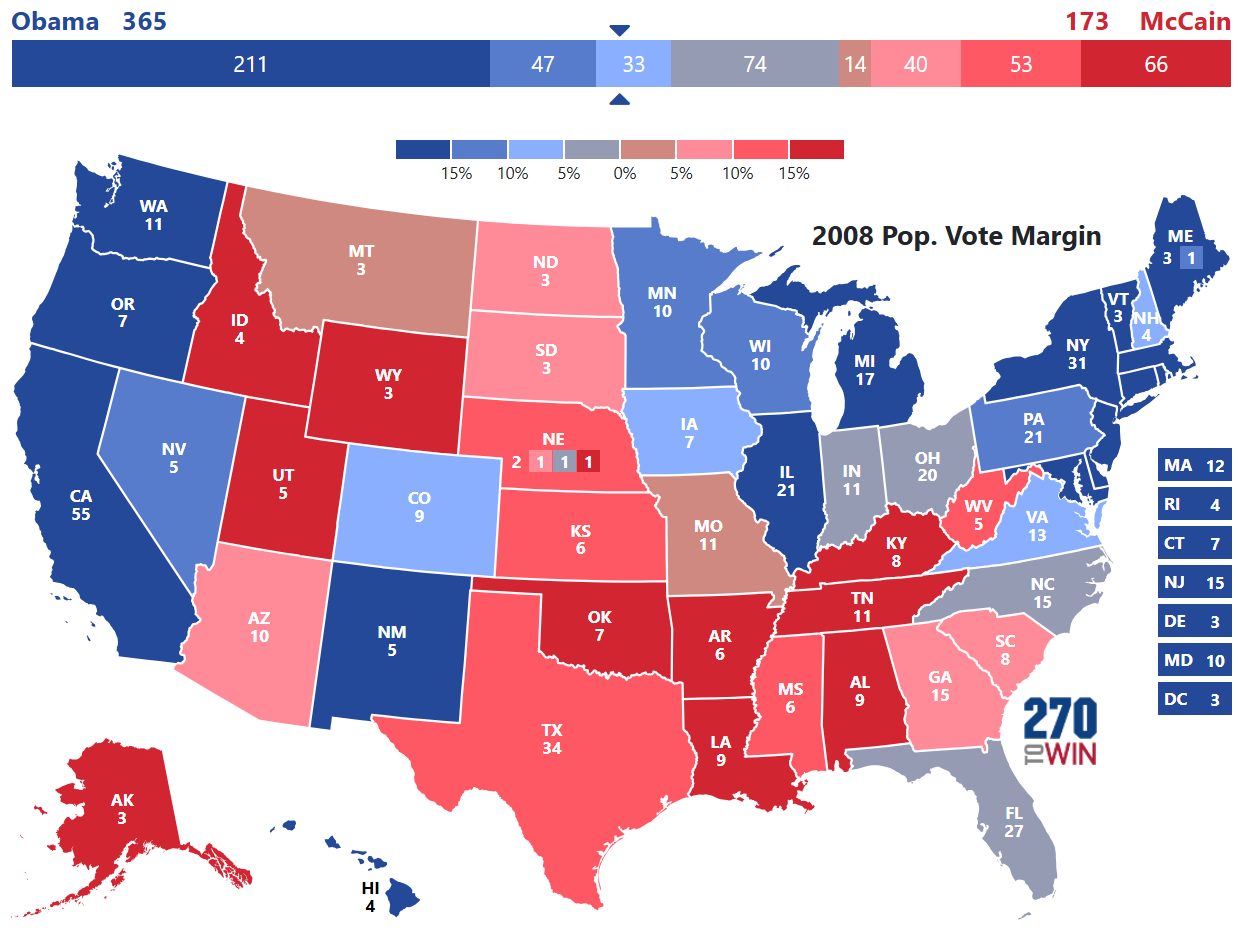
A gradient can be seen when the margin of victory is depicted on a similar map through the use of color shading, as in the figure below (from 270towin.com). Whereas the map above draws each region in either red or blue to indicate the winner, Vanderplei renders the map with a mixture of colors to indicate the proportion of votes received for each candidate in that region.
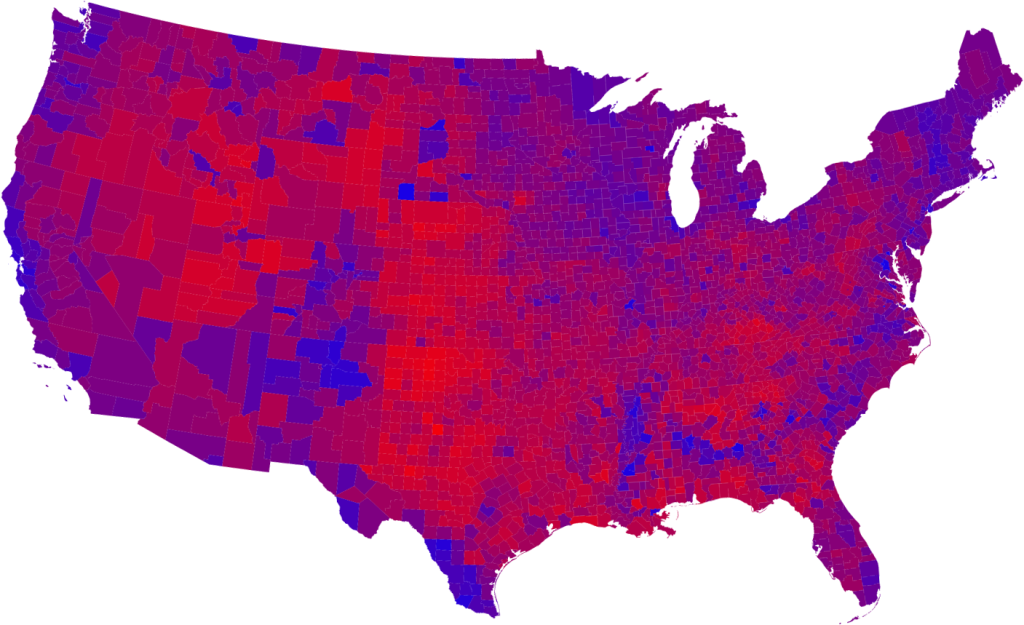
Robert Vanderplei proposed a Purple America map that visualizes the margin of victory with a gradient of colors. In the example below, he draws each region at a county-by-county level instead of a state-by-state level, to depict a more granular gradient.
Kevin Wayne [1] developed a SIGCSE Nifty Assignment in which you will draw this map using GPS coordinates for the regions (states or counties), and then color code those regions using electoral results. The GPS coordinates of each region and the electoral results in those regions will be given to you.
Part 1: Number Systems and RGB Color Coding
Color Coding
To create the color codings, the proportion of votes cast for each of (up to) three candidates is converted into a RGB color. An RGB color is defined by a “tuple,” or collection of values: each value in this 3-tuple represents the proportion of red, blue, and green to be mixed in to the color shown. This is called a 3-tuple because there are three values in the tuple (the red, blue, and green proportion).
We will use 24-bit color in this example, meaning that each of the three values (red, green, and blue) in the tuple can be represented with an 8-bit value.
How many different values can you represent with an 8-bit value? In other words, how many different pure "red" colors are there? There will be an equal number of pure "blue" and pure "green" values as well. (Click to reveal)
Since each of the 8 bits is a binary bit value (0 or 1), there are two possibilities for each of the eight bit fields. Thus, there are \(2^{8}\) different values that can be represented using an 8-bit entry, or 256 distinct shades of pure red, pure blue, or pure green. This includes the colors black (a value of 0) and white (a value of 255).How many different values can you represent with a 24-bit value? In other words, how many different colors can we work with in total? (Click to reveal)
There are \(2^{24}\) or approximately 16 million colors that we can represent as combinations of the 256 possible red values, 256 possible blue values, and 256 possible green values. This is the same as combining three entries of up to 256 possibilities each (the 256 reds, 256 greens, and 256 blues), or \(256^{3}\). By the law of exponents, \(2^{24} = (2^{8})^{3} = 256^{3}\).The color wheel below from Wikipedia shows some example color mixtures. These values are in hexadecimal, so they range from 0x00 to 0xff for decimal values 0 to 255. Here is a guide from Khan Academy to number systems and converting between hexadecimal, binary, and decimal.

Part 2: Drawing Figures
Adding the Princeton stdlib Library to Your Project
The edu.princeton.cs.algs4.StdDraw class contains a library that will draw polygons and other shapes on a window. The coordinates of this window are assumed to range from [0, 1]. This class is contained in the algs4.jar file provided by Robert Sedgewick.
To use this jar, after creating a Gradle Java project in Netbeans, add the following line inside the dependencies section of your build.gradle file:
compile fileTree(dir: 'libs', include: '*.jar')
If you do not have a dependencies section, you can add one as follows:
dependencies {
    compile fileTree(dir: 'libs', include: '*.jar')
}
Now, jar files added to the libs directory of your project will be available for use in your code. Download and copy the algs4.jar file into a subdirectory of your project called libs.
In your program, you can add the following import line at the top:
import edu.princeton.cs.algs4.*;
Basic Drawing Functionality
You can draw arcs and circles using the following methods, once you add the jar to your libs directory (and add the dependency line to your build.gradle file), by calling one of these functions from your program:
// DO NOT COPY THIS PART OF THE CODE - THIS IS JUST A REFERENCE!
// These are like Math.pow() - functions that the jar file provides
// now you have functions called StdDraw.circle and StdDraw.arc, that
// look like the below functions.

// Assumption: the edu.princeton.cs.algs4 package is imported in this file with
// import edu.princeton.cs.algs4.*;

//... then inside your class, and inside main(), you can call these functions:

// x and y are the center coordinates of the circle
// radius is the radius of the circle (or the circle traced by the arc)
// angle1 and angle2 are the angles traced by the arc from the starting and ending points, respectively
//      ... where 0 is the 3 o'clock position, and 90 is 12 o'clock, 180 is 9 o'clock, and 270 is 6 o'clock.
//      ... angle1 is where to start tracing the circle, and angle2 is where to stop.
public static void arc(double x, double y, double radius, double angle1, double angle2)
public static void circle(double x, double y, double radius)
For example, you can draw a circle centered at the middle of the window, with a radius of 0.5 (since the window has dimensions 1 by 1, this circle will take up the whole window):
StdDraw.circle(0.5, 0.5, 0.5); // put this inside your public static void main() function.
StdDraw.arc(0.5, 0.5, 0.4, 90, 270); // this draws a circle inside, but only a semi-circle
Using these methods and examples, try drawing a “happy face” at the center of the window. Recall that the coordinate plane of the window on the x and y axes ranges from 0 to 1, so your coordinates should always be in this range. Your happy face should have a circle for a face, circles for eyes inside, and an arc for the nose and smile. For fun, add some eyebrows with arcs, too!
Part 3: Encapsulating Drawing Functionality in a Function
Creating a Function to Draw a Figure
Now, create a function called drawHappyFace that draws a face centered at coordinates given as function parameters.
Instead of hard-coding the x, y, and radius values for your face, calculate them based on the input parameters. For example, your eyes might have a y value that is equal to the given y parameter plus or minus one-half the radius (this is just an example - feel free to play with the values like this and see where the eyes end up for yourself!). I suggest hard-coding values at first to see the relationship between x, y, and radius, and the ultimate placement of the facial features.
Part 4: Using Iteration to Draw Several Figures
Using a Loop to Draw Multiple Figures
Using a loop in your main function, call drawHappyFace to draw faces at several different positions on the screen.
You might, for example, have a loop like this:
for(int i = 1; i <= 3; i++) { // draw three faces
    // TODO: Compute x and y based on the value of i
    // ... remember that the coordinate plane goes from x = [0, 1] and y = [0, 1]
    // ... so your calculated x and y points should be within 0 and 1

    // TODO: Call drawHappyFace with these values!
}
Part 5: Reading GPS Coordinates for the Polygons
Reading the GPS Coordinates File
Now we can read the GPS coordinates of the regions to be drawn. Each region is a polygon specified by a set of latitude and longitude coordinates. Our goal is to read this file, and create an array of X and Y coordinates from these GPS values to be rendered as polygons by the drawing library we used above. We can pick any color for now to draw these polygons; we’ll specify individual colors for each one later.
A set of GPS coordinates for each county in the United States can be found here. You can use the readFile function below to read a file into an ArrayList of String values (one entry for each line in the file), so that we can parse the entries in this file.
    // import the following at the top and remove the comments:
    // import java.io.BufferedReader;
    // import java.io.FileReader;
    // import java.util.ArrayList;
    // import java.io.IOException;

    /**
     * Read a text file, line by line, into an array of Strings
     * Adapted from https://www.journaldev.com/709/java-read-file-line-by-line
     * @param filePath the full or relative path to the file to be read
     * @param contents an array of Strings, to be populated with for each line read in the file
     * @return the contents parameter, which now contains an array of strings corresponding to the lines read from the file
     * @throws IOException if the file cannot be read (i.e., if it does not exist, or if the user does not have the required permissions to read the file)
     */
    public static String[] readFile(String filePath) throws IOException {
        ArrayList<String> contents = new ArrayList<String>();

        /* https://www.journaldev.com/709/java-read-file-line-by-line */
        BufferedReader reader;
        FileReader fileReader;

        fileReader = new FileReader(filePath);
        reader = new BufferedReader(fileReader);

        String line = reader.readLine();

        while(line != null) {
            contents.add(line);
            line = reader.readLine();
        }

        reader.close();

        String[] result = new String[contents.size()];
        result = contents.toArray(result);
        return result;
    }
Download the county coordinates file and save it in your project directory. I created a subdirectory called data in my project directory and saved it there. Use the readFile function to read this file (the path to this file is ./data/USA-county.txt if you used a subdirectory called data like I did).
The file is formatted as follows:
File Header
The first three lines of the file are the coordinates of the top left and bottom right used on the map, followed by the number of regions in the file. Notice that Latitude and Longitude are separated by three spaces.
Latitude   Longitude
Latitude   Longitude
Count of the Number of Regions
<blank line>
Region
Each region is then displayed using the same format:
Region Name
State Abbreviation
Count of the Number of Polygon Latitude/Longitude corners`
 Latitude   Longitude
 Latitude   Longitude
 Latitude   Longitude
 ...
 Latitude   Longitude
 <blank line>
The region name (for example, the name of the county) is followed by the state name (for example, PA for Pennsylvania), followed by the number of coordinates. Like before, Latitude and Longitude are separated by three spaces, but there is also a space at the beginning of each Latitude/Longitude line.
Parsing the Region File
Loop through the array, reading each line of text, and generate two arrays of doubles for each region. These arrays (x and y) will contain the latitude/longitude coordinates of the polygon defined by each region in the file. Every time you read a new region (from the start of the region all the way to a blank line indicating the end of the region), create a HashMap to store the values for that region. The HashMap should map a String (the region name) to a HashMap<String, Double[]> to contain the coordinates:
- RegionName: a String containing the name of the region
- Coordinates: another HashMap containing the GPS latitude and longitude coordinates
The Coordinates HashMap should map a String to a Double[] or an ArrayList<Double>, containining the following keys:
- x: an array of
Doublevalues containing the array of x coordinates of the polygon - y: an array of
Doublevalues containing the array of y coordinates of the polygon
Note that you will need to remove the extra spaces within the Strings that you read, and “tokenize” the Latitude and Longitude values from each line (since both coordinates appear on each line of text). The following functions will help you do this:
String.split(String delimiter): return an array of Strings, with one entry for word or “token” on the input String object on which split is called, where each word is separated by a “delimiter” given in the method parameter (note that our coordinate sare separated or delimited by three spaces)String.strip(): return a new string that is the original string being called upon but with any leading or trailing whitespace removedString.length(): Return an integer for the length of a string
How would you know if you have reached a newline in the file, and are thus finished reading a region? (Click to reveal)
Each region is separated by a newline. After removing whitespace from the line, the length of a blank line will be 0. You can use the `String.strip()` method to remove leading and trailing whitespace from a string, for example: `line = line.strip();`.Then, you will need to convert the Latitude/Longitude coordinates from a String to a double. The standard library function Double.parseDouble() will do this for you, by taking a String parameter and returning its numeric value as a double.
Part 6: Scaling the Coordinates to a Graphical Plane
Converting the Latitude / Longitude Values to a [0, 1] Coordinate Plane
If you know the largest and smallest X,Y values from the whole file (hint: you do!), you can call these maxX and maxY, and compute the relative position on a [0,1] coordinate plane.
How would you convert between absolute coordinates and a relative [0, 1] scale? (Click to reveal)
Each position is the relative distance on the X or Y axis as a ratio to the absolute distance represented on the original map. So, a point (25, 50) on a [0, 100] coordinate scale would be 25% of the way across, and 50% of the way down that map. This is obtained by dividing the coordinate value by the range on that axis (here, 100). To account for negative coordinates (which can happen when using GPS coordinates!), we first subtract the minimum X and Y value on the map before computing this ratio. The resulting value can be multiplied by the new range, but since we are using a [0, 1] projection, the new scale is 1, and there is no need to scale back up. The formulae to scale GPS coordinates to a [0, 1] X/Y map are as follows:\(y = \frac{y - minY}{maxY - minY}\)
\(x = \frac{x - minX}{maxX - minX}\)
Drawing a Custom Polygon using an Array of Coordinates
Earlier, we drew circles and rectangles on the screen using x and y coordinates. We can also draw custom polygons by providing the x and y coordinate of each corner (that is, where to draw each line of the polygon). We can specify all the x and all the y coordinates at once using an array, which combines all the x and y points into a single variable. Here is an example that you can try:
// Assumption: the edu.princeton.cs.algs4 package is imported in this file with
// import edu.princeton.cs.algs4.*;
// import java.awt.Color;

//... then you can do this:

// This is the RGB color of the polygon
int red = 0;
int green = 0;
int blue = 0;

/* x and y is an array of coordinates of the corners of the polygon -
the polygon will be automatically closed by connecting the last point
to the first point.  Here, the points are
(0, 0), (0.2, 0), (0.2, 0.2), (0, 0.2),
and, finally, back to (0, 0) automatically.
You will replace this with your own arrays.
Do not copy these x and y arrays - you'll use paramters instead! */
double[] x = {0, .2, .2, 0 };
double[] y = {0,  0, .2, .2};

Color color = new Color(red, green, blue);

StdDraw.setPenRadius(); // This resets the pen thickness to the default
StdDraw.setPenColor(color);
StdDraw.filledPolygon(x, y);
StdDraw.filledPolygon takes in an array of doubles (double[]). If you are using an ArrayList<Double>, you can convert it to a double[] by pasting and calling this function into your program:
// call this with:
// double[] xArr = toArray(x);
// where x is an ArrayList<Double>
// and you can pass x to filledPolygon (repeat for y!)
public static double[] toArray(ArrayList<Double> arr) {
        // Make an array big enough to hold everything in the ArrayList
        double[] result = new double[arr.size()];

        // now copy each value!
        for(int i = 0; i < arr.size(); i++) {
            result[i] = arr.get(i);
        }

        return result;
}
What to Do
When you parse your coordinate file, notice that the minimum and maximum latitude and longitude coordinates are given at the top of the file. Read them prior to your loop and store them as your minX, minY, maxX, and maxY values.
Now that you have an array of x and y coordinates scaled from 0 to 1, you can draw on the screen using these polygons! Pass the arrays to filledPolygon using the code snippet above (replacing the array we gave you) to draw each region in the country. Better yet, you can make a function to do this, so that you can pass the array for each region and draw them one by one! Write a function that takes an ArrayList<Double> and draws the polygon using the above code snippet. Let’s call it drawRegion(ArrayList<Double> x, ArrayList<Double> y)
Then, in a loop, iterate over your HashMap set of counties to obtain the coordinates, and scale them to a 0 to 1 plane using the math formulas to scale according to the minimum and maximum x and y in the file (see above!). Create new ArrayLists for the scaled values, or modify the values directly in your x and y arrays. Pass the scaled x and y ArrayLists to the drawRegion polygon drawing function you wrote just above. Try passing these newly scaled x and y coordinate arrays to your polygon drawing function; they should now render (albeit in a single color).
Part 7: Generating Color Codes from Electoral Votes
Reading the Electoral Votes File and Generating the Color Codes
Coordinate data for other geographic regions (for example, a state-by-state map of the United States, or a map of each state by county) can be found here. In addition, this file contains the election results for a given year (for example, USA1968.txt for the state-by-state presidential election in 1968, or PA2008.txt for the county-by-county presidential election results in Pennsylvania in 2008). The format of this file is a Comma Separated Value (CSV) file, meaning that each token on a line is separated by a comma character (as opposed to spaces which we used earlier). The first line is a header line, giving the labels for each column in the file (for example, the name of each candidate). This can be ignored; each subsequent line contains:
State Name,Candidate 1 Votes,Candidate 2 Votes,Candidate 3 Votes
If you are drawing each county, you’ll need to open up the file named as the abbreviated state followed by the election year you’re interested in. For example, Alabama in 2004 would be AL2004.txt. Fortunately, you will know the abbreviated state name: recall that it is included in the GPS file you read earlier, and you saved it in the HashMap you created! If you loop over each of these HashMaps, you can open the correct file given the abbreviated state name, and then read the election results file using a similar approach to the one you took when reading the GPS coordinates file. This time, the tokens are delimited by commas instead of spaces.
When you define the color of each county region earlier, compute the red, green, and blue ratios based on the following formula:
\(colorConcentration_{c = candidate} = \frac{votes_{c}}{\sum_{i \in candidates} votes_{i}}\)
That is, the concentration of a color is the ratio of total votes received by the candidate represented by that color. Multiply that ratio by 255 and convert to an integer, and you have the RGB entry for that region. Repeat this for red, green, and blue (one color for each candidate), and you have a complete color definition for that region! In our filledPolygon code example above, where are the red, green, and blue color values set? Make the colors parameters to your function to draw a polygon, and specify them using the red, green, and blue colorConcentration values you just computed! Each region should now render on your screen using a color that blends the votes cast for each candidate from that region.
Render the map using margin-of-victory color shading for the election of your choice.
Extra Credit (10 Points Each)
Extra Credit 1: Only Read the File Once: Using a Cache for Better Performance
You may have noticed that it was necessary to open and read each election results file more than once (for example, once for every county you encounter). You can avoid this by storing the electoral file in memory every time you read it. This is known as creating a “cache” and will allow your program to run much faster, since disk I/O operations are much slower than other computations.
How might a dictionary allow you to check if a file has been read yet, and then to read it if necessary? (Click to reveal)
The state or filename could be the dictionary "key;" if the key is not present in the dictionary, then the file has not yet been read. Once the data has been read from the file, it can be inserted into the dictionary under that key. Next time the file is needed, the key will be present in the dictionary, and the data can be accessed without re-reading the file. In other words, the file must be read only if the data is not in the dictionary. After reading the file (once), the data is stored in the dictionary for subsequent use.Extra Credit 2: Rendering a Different Map
Create or read a map GPS coordinates for another region, and render it. Think of another gradient visualization you can perform. As long as you store your data in the same way as we did for this assignment, this program can be re-used for other visualizations without much if any additional effort!
Extra Credit 3: Rendering with a Mercatur Projection
You may have noticed that the map of the United States appears somewhat distorted because it is projected on a square map. Lines of latitude and longitude are rounded due to the curvature of the Earth. Two-dimensional renderings often use a projection to distort the map in order to better render this curved surface on a rectangular 2D projection. One such projection is a Mercatur Projection. Such projections must move the projection inaccuracies somewhere (since we are projecting a 3D surface onto a 2D one, some information must necessarily be lost somewhere!). Mercatur projections exaggerate features at the extremes of the projection (that is, the top and bottom). This is why Alaska and Greenland appear larger than they really are when projected in this way. Howeve,r this better depicts the curvature of the other features of the map, including that of the United States.
Prior to scaling your coordinates to a [0,1] plane, your latitude and longitude values can be projected via a Mercatur Projection using the following approach (from https://gis.stackexchange.com/questions/298619/mercator-map-coordinates-transformation-formula). It assumes that you know the latitude and longitude of the origin point, the top left point, and the bottom right point, as well as the latitude and longitude of the point you wish to project. (Click to reveal)
let a = 6378137 (equatorial radius in meters)let MercaturX1 = \(a \times topLeftLongitude\)
let MercaturY1 = \(a \times ln(tan(\frac{\pi}{4} + \frac{topLeftLatitude}{2}))\)
let MercaturX2 = \(a \times bottomRightLongitude\)
let MercaturY2 = \(a \times ln(tan(\frac{\pi}{4} + \frac{bottomRightLatitude}{2}))\)
let MercaturDistance = \(\sqrt{(MercatorX2 - MercatorX1)^{2} + (MercatorY2 - MercatorY1)^{2}}\)
let DistanceMap = \(\sqrt{(bottomRightLongitude - topLeftLongitude)^{2} + (bottomRightLatitude - topLeftLongitude)^{2}}\)
let ScaleFactor = \(\frac{MercatorDistance}{DistanceMap}\)
let MercatorX0 = \(a \times originLongitude\)
let MercaturY0 = \(a \times ln(tan(\frac{\pi}{4} + \frac{originLatitude}{2}))\)
let projectedLatitude = \(2 \times atan(exp(\frac{ScaleFactor \times -(latitude) + MercatorY0}{a})) - \frac{\pi}{2}\)
let projectedLongitude = \(\frac{ScaleFactor \times x + MercatorX0}{a}\)
After projecting all of your coordinates, you can scale them to a [0, 1] plane as before.
Extra Credit 4: Improving Accessibility
One of the challenges associated with producing visualizations is that they may not be universally productive and accessible. For example, those with visual impairments will not benefit from this visualization. Choose a color contrast palette with better contrast (cite any sources used when identifying such color palettes), and add a textual represnetation in the middle of each state (or pointing to the state) that indicates the percentage and winner in that state.
-
Nick Parlante, Julie Zelenski, Josh Hug, John Nicholson, John DeNero, Antti Laaksonen, Arto Vihavainen, Frank McCown, and Kevin Wayne. 2014. Nifty assignments. In Proceedings of the 45th ACM technical symposium on Computer science education (SIGCSE ’14). Association for Computing Machinery, New York, NY, USA, 621–622. DOI:https://doi.org/10.1145/2538862.2538995 ↩
Submission
If you wrote code as part of this assignment, please include a README in which you describe your design, approach, and implementation. Additionally, please answer any questions from the assignment, and include answers to the following questions:- If collaboration with a buddy was permitted, did you work with a buddy on this assignment? If so, who?
- Approximately how many hours it took you to finish this assignment (I will not judge you for this at all...I am simply using it to gauge if the assignments are too easy or hard)?
- Your overall impression of the assignment. Did you love it, hate it, or were you neutral? One word answers are fine, but if you have any suggestions for the future let me know.
- Any other concerns that you have. For instance, if you have a bug that you were unable to solve but you made progress, write that here. The more you articulate the problem the more partial credit you will receive (it is fine to leave this blank).
Assignment Rubric
| Description | Pre-Emerging (< 50%) | Beginning (50%) | Progressing (85%) | Proficient (100%) |
|---|---|---|---|---|
| Algorithm Implementation (60%) | The algorithm fails on the test inputs due to major issues, or the program fails to compile and/or run | The algorithm fails on the test inputs due to one or more minor issues | The algorithm is implemented to solve the problem correctly according to given test inputs, but would fail if executed in a general case due to a minor issue or omission in the algorithm design or implementation | A reasonable algorithm is implemented to solve the problem which correctly solves the problem according to the given test inputs, and would be reasonably expected to solve the problem in the general case |
| Code Quality and Documentation (30%) | Code commenting and structure are absent, or code structure departs significantly from best practice, and/or the code departs significantly from the style guide | Code commenting and structure is limited in ways that reduce the readability of the program, and/or there are minor departures from the style guide | Code documentation is present that re-states the explicit code definitions, and/or code is written that mostly adheres to the style guide | Code is documented at non-trivial points in a manner that enhances the readability of the program, and code is written according to the style guide |
| Writeup and Submission (10%) | An incomplete submission is provided | The program is submitted, but not according to the directions in one or more ways (for example, because it is lacking a readme writeup) | The program is submitted according to the directions with a minor omission or correction needed | The program is submitted according to the directions, including a readme writeup describing the solution |